Understanding and Implementing Speech Recognition using HMM

10 min readDec 15, 2018

The first step in implementing Speech recognition is understanding how audio data works?

sampling frequency

The sampling frequency (or sample rate) is the number of samples per second in a Sound. For example: if the sampling frequency is 44100 hertz, a recording with a duration of 60 seconds will contain 2,646,000 samples

All audio files are sampled at a sampling frequency of 44100

Reading Audio File

Generally, audio files are treated as wave files and while reading an audio file we get sampling frequency and the actual audio

Let’s read an audio file which is 3 seconds long

import numpy as np
import matplotlib.pyplot as plt
from scipy.io import wavfile
sampling_freq, audio = wavfile.read('./input_read.wav')
print( '\nShape:', audio.shape)
print ('Datatype:', audio.dtype)
print ('Duration:', round(audio.shape[0] / float(sampling_freq), 3), 'seconds')
_____________________________________
('\nShape:', (132300,))
('Datatype:', dtype('int16'))
('Duration:', 3.0, 'seconds')

from above results we can see that for each millisecond there is an amplitude which is a 16-bit signed integer(1-bit for sign and 15-bits long integer)

Now let’s normalize audio data and plot a sample data on time axis

audio=audio/2.**15
audio=audio[:30]
x_values = np.arange(0, len(audio), 1) / float(sampling_freq)
x_values *= 1000
plt.plot(x_values, audio, color='black')
plt.xlabel('Time (ms)')
plt.ylabel('Amplitude')
plt.title('Audio signal')
plt.show()

As the above signal is in time domain we can use simple Fourier transform and transform it into frequency domain but what are Fourier transforms

The Fourier Transform is a tool that breaks a waveform (a function or signal) into an alternate representation, characterized by sine and cosines. The Fourier Transform shows that any waveform can be re-written as the sum of sinusoidal functions

Virtually everything in the world can be described via a waveform — a function of time, space or some other variable. For instance, sound waves, electromagnetic fields, the elevation, the price of y stock versus time, etc. The Fourier Transform gives us a unique and powerful way of viewing these waveforms.

transformed_signal = np.fft.fft(audio)

FFTs take a waveform of complex numbers (eg, [.5+.1j, .4+.7j, .4+.6j, …]) to another sequence of complex numbers

It turns out that if the input waveform is real instead of complex, then the FFT has a symmetry about 0, so only the values that have a frequency >=0 are uniquely interesting.

The values output by the FFT are complex, so they have a Real and Imaginary part, but this can also be expressed as a magnitude and phase. For audio signals, it’s usually the magnitude that’s the most interesting, because this is primarily what we hear. Therefore people we can use abs (which is the magnitude), but the phase can be important for different problems as well.

half_length = np.ceil((len_audio + 1) / 2.0)
half_length=int(half_length)
transformed_signal = abs(transformed_signal[0:half_length])
transformed_signal **= 2

Now we get the power of the signal by extracting the FFT values in decibels magdB = 20 * math.log10(abs(STFT)) and plotting frequency vs power

power = 20 * np.log10(transformed_signal)
x_values = np.arange(0, half_length, 1) * (sampling_freq / len_audio) / 1000.0)
plt.figure() plt.plot(x_values, power, color='black')
plt.xlabel('Freq (in kHz)')
plt.ylabel('Power (in dB)')
plt.show()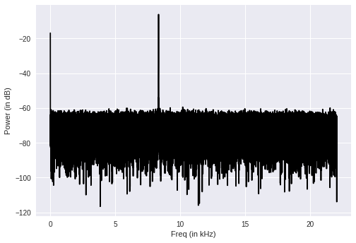

let’s generate our own audio

to generate a sound wave we can take a sinusoidal function along the time axis with a constant frequency y=sin(2π.f.t ) with some noise

duration = 3
sampling_freq = 44100
tone_freq = 587
min_val = -2 * np.pi
max_val = 2 * np.pi 
t = np.linspace(min_val, max_val, duration * sampling_freq)
audio = np.sin(2 * np.pi * tone_freq * t)
noise = 0.4 * np.random.rand(duration * sampling_freq)
audio += noise
scaling_factor = pow(2,15) - 1
audio_normalized = audio / np.max(np.abs(audio))
audio_scaled = np.int16(audio_normalized * scaling_factor)
x_values = np.arange(0, len(audio), 1) / float(sampling_freq)
x_values *= 1000
plt.plot(x_values, audio, color='red') 
plt.xlabel('Time (ms)')
plt.ylabel('Amplitude')
plt.title('Audio signal')
plt.show()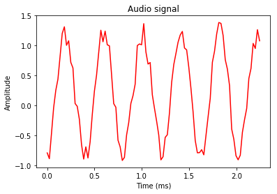

# Saving the generated Audio file
output_file = 'output_generated.wav'
write(output_file, sampling_freq,audio_scaled)

Feature Extraction From an Audio File

While building a speech recognition system first thing is we have to extract the important features and discard the noise

Generally sound produced by humans is shaped by the vocal cords in the mouth, human vocal tract give out the envelope of the short time POWER-SPECTRUM like exactly we have plotted in one of the above diagrams (frequency VS power) and we use the Mel Frequency Cepstral Coefficient (MFCC) to accurately represent this envelope of SPECTRUM

How to extract Mel Frequency Cepstral Coefficient(MFCC)

Frame the signal into short frames.
For each frame calculate the periodogram estimate of the power spectrum.
Apply the mel filterbank to the power spectra, sum the energy in each filter.
Take the logarithm of all filterbank energies.
Take the DCT of the log filterbank energies.
Keep DCT coefficients 2–13, discard the rest.

An audio signal is constantly changing, This is why we frame the signal into 20–40ms frames. The next step is to calculate the power spectrum of each frame. This is motivated by the human cochlea (an organ in the ear) which vibrates at different spots depending on the frequency of the incoming sounds This effect becomes more pronounced as the frequencies increase. For this reason, we take clumps of speech bins and sum them up to get an idea of how much energy exists in various frequency regions, This is performed by our Mel filterbank, We are only interested in roughly how much energy occurs at each spot. The Mel scale tells us exactly how to space our filterbanks and how wide to make them

What is the Mel scale?

The Mel scale relates perceived frequency, or pitch, of a pure tone to its actual measured frequency. Humans are much better at discerning small changes in pitch at low frequencies than they are at high frequencies. Incorporating this scale makes our features match more closely what humans hear. The formula for converting from frequency to Mel scale is:

M(f)=1125*ln(1 + f/700)

The final step is to compute the DCT (Discrete cosine transform) of the log filterbank energies. There are 2 main reasons this is performed. Because our filterbanks are all overlapping, the filterbank energies are quite correlated with each other. The DCT decorrelates the energies which means diagonal covariance matrices can be used to model the features in e.g. an HMM (Hidden Markov Models) classifier

What is DCT?

Like any Fourier-related transform, discrete cosine transforms (DCTs) express a function or a signal in terms of a sum of sinusoids with different frequencies and amplitudes. Like the discrete Fourier transform (DFT), a DCT operates on a function at a finite number of discrete data points. The obvious distinction between a DCT and a DFT is that the former uses only cosine functions, while the latter uses both cosines and sines (in the form of complex exponentials). However, this visible difference is merely a consequence of a deeper distinction: a DCT implies different boundary conditions from the DFT or other related transforms.

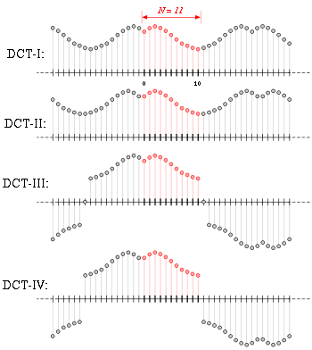
https://en.wikipedia.org/wiki/Discrete_cosine_transform

The best part is there is a package called librosa to extract MFCC features

from librosa.feature import mfcc
import librosa
sampling_freq, audio = librosa.load("input_freq.wav")
mfcc_features = mfcc(sampling_freq,audio)
print(\nNumber of windows =', mfcc_features.shape[0])
print('Length of each feature =', mfcc_features.shape[1])
-------------------------------------
Number of windows = 20
Length of each feature = 18

Plotting the MFCC Features

mfcc_features = mfcc_features.T
plt.matshow(mfcc_features)
plt.title('MFCC')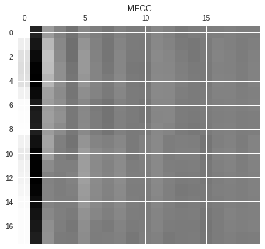

Hidden Markov Models(HMM)

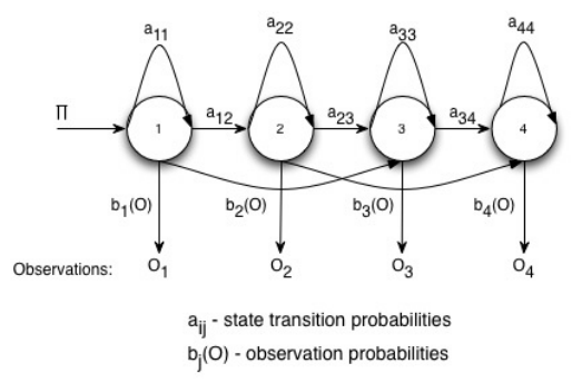
Hidden Markov Models (HMMs). The HMM is a generative probabilistic model, in which a sequence of observable X variables is generated by a sequence of internal hidden states Z. The hidden states are not observed directly. The transitions between hidden states are assumed to have the form of a (first-order) Markov chain. They can be specified by the start probability vector π and a transition probability matrix A. The emission probability of an observable can be any distribution with parameters θ conditioned on the current hidden state. The HMM is completely determined by π, A and θ.

Markov chains (and HMMs) are all about modeling sequences with discrete states. Given a sequence, we might want to know e.g. what is the most likely character to come next, or what is the probability of a given sequence. Markov chains give us a way of answering this question. To give a concrete example, you can think of text as a sequence that a Markov chain can give us information about e.g. ‘THE CAT SA’. What is the most likely next character

Why choosing HMM ?

Markov chains only work when the states are discrete. speech satisfies this property since there are a finite number of mfcc features in a sequence. If you have a continuous time series then Markov chains can’t be used.

in speech recognition. The states are phonemes i.e. a small number of basic sounds that can be produced. The observations are frames of audio which are represented using MFCCs. Given a sequence of MFCCs i.e. the audio, we want to know what the sequence of phonemes was. Once we have the phonemes we can work out words using a phoneme to word dictionary. Determining the probability of MFCC observations given the state is done using Gaussian Mixture Models (GMMs).

https://en.wikipedia.org/wiki/Hidden_Markov_model

Now we are good to go and implement speech recognition from scratch you can find the data to be used for this code at click here to download datasets

OBJECTIVE

given the voice of a fruit, we have to predict the name of the fruit

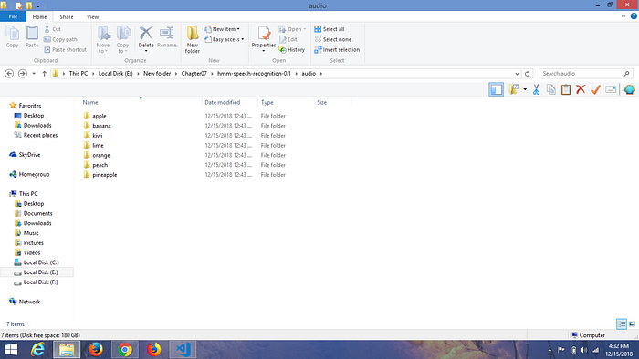
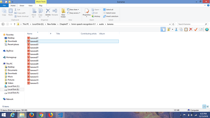
Files hierarchy is shown in the above images we have 7 files of fruit names voice data, there are 15 recordings corresponding to each of fruits file

for dirname in os.listdir(input_folder):
  subfolder = os.path.join(input_folder, dirname)
  label = subfolder[subfolder.rfind('/') + 1:]
  print(label)________________________________________________lime 
orange
peach 
kiwi 
apple 
pineapple 
banana!pip install hmmlearn
!pip install features
import os
import numpy as np
from scipy.io import wavfile 
from hmmlearn import hmm #importing GaussianHMM 
import librosa # reading wavefilesfrom librosa.feature import mfcc #to extract mfcc features

How to train a GaussianHMM Model

We will train a GaussianHMM for each of our fruit kinds, which means we train 7 GaussianHMM models, and during the Testing time we pass our audio file into all 7 GaussianHMM models and we get a score from each of a model and we can give the label corresponding to the model with maximum score

as we have to train seven GaussianHMM models and store them we will write a class called HMMTrainer

Now let’s write a class for GaussianHMM as a constructer along with two functions one to train the model train and the other to get the score on test data get_score

class HMMTrainer(object):
   def __init__(self, model_name='GaussianHMM', n_components=4):
     self.model_name = model_name
     self.n_components = n_components

     self.models = []
     if self.model_name == 'GaussianHMM':
        self.model=hmm.GaussianHMM(n_components=4)
     else:
        print("Please choose GaussianHMM")   def train(self, X):
       self.models.append(self.model.fit(X))   def get_score(self, input_data):
       return self.model.score(input_data)

Now let’s start iterating over each fruit file, the label for each of the 15 recordings is the parent file so we can extract the label from the parent file

hmm_models = []
for dirname in os.listdir(input_folder):
  # Get the name of the subfolder 
  subfolder = os.path.join(input_folder, dirname)
  if not os.path.isdir(subfolder): 
    continue
  # Extract the label
  label = subfolder[subfolder.rfind('/') + 1:]
  # Initialize variables
  X = np.array([])
  y_words = []

In each fruit file, there are 15 recordings so we can use 14 files of each fruit as train data and one for the test data, now by iterating over each wave file, we can get mfcc features for every fruit file, but we are choosing only the first 15 mfcc features for each wave file

for filename in [x for x in os.listdir(subfolder) if x.endswith('.wav')][:-1]:
   # Read the input file
   filepath = os.path.join(subfolder, filename)
   sampling_freq, audio = librosa.load(filepath)
   # Extract MFCC features
   mfcc_features = mfcc(sampling_freq, audio)
   # Append to the variable X
   if len(X) == 0:
     X = mfcc_features[:,:15]
   else:
     X = np.append(X, mfcc_features[:,:15], axis=0)
   # Append the label
   y_words.append(label)print('X.shape =', X.shape)___________________________________________________________________X.shape = (280, 15) 
X.shape = (280, 15) 
X.shape = (280, 15)
X.shape = (280, 15)
X.shape = (280, 15)
X.shape = (280, 15)
X.shape = (280, 15)

after extracting mfcc features from each of the fruit files we can train HMMTrainer by initializing the class and we will do this for all fruit files

hmm_trainer = HMMTrainer()
hmm_trainer.train(X)
hmm_models.append((hmm_trainer, label))
hmm_trainer = None

Now Let’s Test our model

selecting some files from test files

input_files = [
'./hmm-speech-recognition-0.1/audio/pineapple/pineapple15.wav',
'./hmm-speech-recognition-0.1/audio/orange/orange15.wav',
'./hmm-speech-recognition-0.1/audio/apple/apple15.wav',
'./hmm-speech-recognition-0.1/audio/kiwi/kiwi15.wav'
]

Extracting mfcc features for each of the test files

we will get the score for each of the labels for every test file (Recording) so we can take the label corresponding to the maximum score and will be our final prediction.

scores=[]
for item in hmm_models:
  hmm_model, label = item
  score = hmm_model.get_score(mfcc_features)
  scores.append(score)
  index=np.array(scores).argmax()
  # Print the output
  print("\nTrue:", input_file[input_file.find('/')+1:input_file.rfind('/')])
  print("Predicted:", hmm_models[index][1])_________________________________________Results:True: hmm-speech-recognition-0.1/audio/pineapple
Predicted: pineappleTrue: hmm-speech-recognition-0.1/audio/orange
Predicted: orangeTrue: hmm-speech-recognition-0.1/audio/apple
Predicted: appleTrue:hmm-speech-recognition-0.1/audio/kiwi
Predicted: kiwi

Find code implementation

MaharshiYeluri01/SpeechRecognition

Contribute to MaharshiYeluri01/SpeechRecognition development by creating an account on GitHub.

github.com